During your time working in the SEO industry, it’s almost inevitable you’re going to be playing around in Excel. The problem arises when you spend hours trying to manually manipulate your data, instead of using a handy formula that you just didn’t know existed.

Today I’m going to share a few formulas that will help you harness a fraction of Excel’s capabilities and as a result, save you and your company precious time.

All of the examples are performed using a Mac, but it is the same process for both PC and Mac.

Tip 1: How to remove trailing slashes

There are many instances in the day of an SEO where you need to tidy up a hefty list of URLs. One problem is removing all of those pesky forward slashes from the end of URLs. Done manually, this would be a painful process, but fortunately for us there’s a formula to help out! Don’t panic, it’s not important to understand the formula. You can just Copy + Paste (and you’ll still look like a magician)!

=IF(RIGHT(A2,(LEN(A2)-(LEN(A2)-1)))=”/”,LEFT(A2,(LEN(A2)-1)),A2)

1) Copy the formula above into the cell next to your URL (see example) ensuring it references that cell (change the ‘A2’s in formula if needed) and press enter.

2) Copy and Paste the formula down to remove the slashes from your URLs. If the URL has no slash at the end, no change will be made.

How simple was that?

Tip 2: How to capitalise all words in a cell

The =PROPER function will enable you to capitalise the letter of every word in a cell, giving you more time to spend on that in-depth keyword research! I often use this when writing title tags because most keyword exports give you lowercase words.

Here’s how you do it (it’s really easy):

1) Write the formula in an adjacent cell, referencing the cell you want to capitalise: =PROPER(A1)

2) Press enter and Copy and Paste this formula down for all the rows you want to capitalise.

And you’re done. Easy, right?

Tip 3: How to combine multiple cells into one

You can combine multiple cells into one on Excel using numerous methods, manually typing them being the worst option! In the following example we have a list of experienced SEOs by first and last name that we want to be in the same cell.

My preferred method is to use the ‘Concatenate’ function and it’s extremely simple to use:

1) Enter the formula into an adjacent column (insert new column if necessary) referring to all the cells you want to combine – just separate each cell with a comma. In the example below we refer to cell ‘A2’ and ‘B2’.

=CONCATENATE(

2) End the formula with a closing bracket ‘)’, press enter, and Copy and Paste down for all rows you want to combine.

Optional: In some cases (like this one), you may want to include a space, comma or any other punctuation in between your combined words. To do this you just need to adapt the formula to include an extra argument between your referenced cells.

3) Change the formula to: =CONCATENATE(A2,” “,B2)

You are telling the formula that you want to include something between the double quotes, in this case a space.

4) As before, press enter and copy down for all rows to give you your combined cell looking exactly how you wanted it to!

NOTE: The Concatenate function can combine as many cells as you want. Just keep adding more arguments separated by commas.

Tip 4: How to split one cell into multiple columns of data

As well as the need to combine cells, I regularly find myself splitting them up too. For example, if you have a list of web addresses and you just want the business names then the easiest thing to do is use ‘Text to Columns’ in Excel.

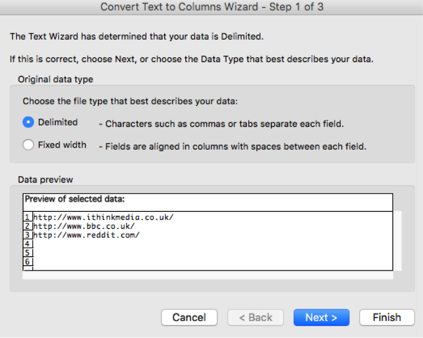
1) Firstly, you need to highlight any data that you want to convert into columns. Click on the ‘Data’ ribbon to find the ‘Text to Columns’ button.

You will then be presented with the following display:

2) In this case we use the ‘Delimited’ option allowing us to choose a character to determine where to separate each column. Click next.

(‘Fixed width’ enables you to manually select where you want the split)

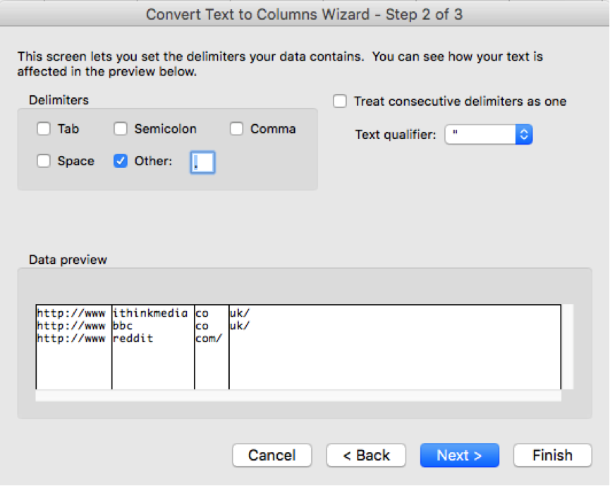
3) Choose the delimiter you require. In this case we are using a full stop, so select the ‘Other’ checkbox and insert a full stop. You can check that the data is being split how you want by looking at the preview (see above).

When you are happy with the preview click ‘Finish’.

(If you were to click ‘Next’ instead of ‘Finish’ this allows you to choose the formats of each new column you are creating)

Optional: To finish, you may want to tidy up the sheet by deleting/hiding any unnecessary columns to just leave you with a list of business names.

You’ve made it to the end of this instalment of Excel tips for SEOs. The key takeaway here is the amount of time you can save by learning just a few simple tricks! My personal tip is perseverance; excel formulas can seem daunting at first, but once you’ve used them a couple of times in practice it becomes second nature.

If anyone has any questions about the tips in this post or would like to know how to use any other functions, just comment and let me know.

Stay tuned for more tips coming soon.